A couple weeks back a blog post was released on the PyTorch blog describing the Stochastic Weight Averaging (SWA) algorithm and it's implementation in pytorch/contrib. The algorithm itself seemed embarrassingly straightforward and relied on averaging snapshots of the the model across a certain learning rate schedule. The authors argued that "SGD tends to converge to the boundary of the low-loss region, making it susceptible to the shift between train and test error surfaces". The hope is that by averaging multiple solutions we'll end up in the center of a flat and wide region of loss (which hopefully should lead to better generalization). I ended up trying this on some semantic parsing tasks I was working on and after a painful couple of hours of manual hyper-parameter selection I ended up with a model that was giving me around 5-10% of relative improvement on a hidden test set.
I was surprised that such a simple modification to the learning algorithm could give such non-trivial gains, which led me to diving deeper into the why. Personally, the most interesting part of the SWA paper was the following excerpt
SGD generally converges to a point near the boundary of the wide flat region of optimal points.
The logic behind the SWA algorithm relies on this statement being true and therefore seemed like a good starting pointer for deeper exploration.
Ornstein-Uhlenbeck Process
The next couple of sections will be slightly out of order. First we'll introduce what the Ornstein-Uhlenbeck process is as well as describe some of the properties it exhibits. Next we'll show that under certain assumptions we can represent SGD as the respective process and finally we'll connect it all back to SWA (hopefully). So what is the OU Process? The clearest intuitive explanation I've heard is that it's a continuous random walk with a tendency to walk toward some centralized point.
Let's define a n-dimensional real vector $\bf{x}_t \in \mathbf{R}^n$ and two square real matrices of the same size $\beta, \Sigma \in \mathbf{R}^{n \times n}$. The OU process is then a stochastic differential equation of the following form $$ d\bf{x}_t= -\beta \bf{x}_t dt + \Sigma d \bf{W}_t $$ where $\bf{W}_t$ is the n-dimensional Wiener process.
Recall that the one dimensional Wiener process is a continuous process starting from 0 satisfying two additional constraints:
- Gaussian Increments: $W_{t+k} - W_{t} = \mathbb{N}(0, k)$
- Independence: $(W_{t+k} - W_{t}) \perp W_j \mid j \le t$
Then an n-dimensional Wiener process is $W(\cdot) = (W^1(\cdot),...,W^n(\cdot))$
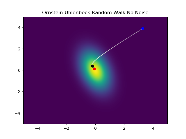
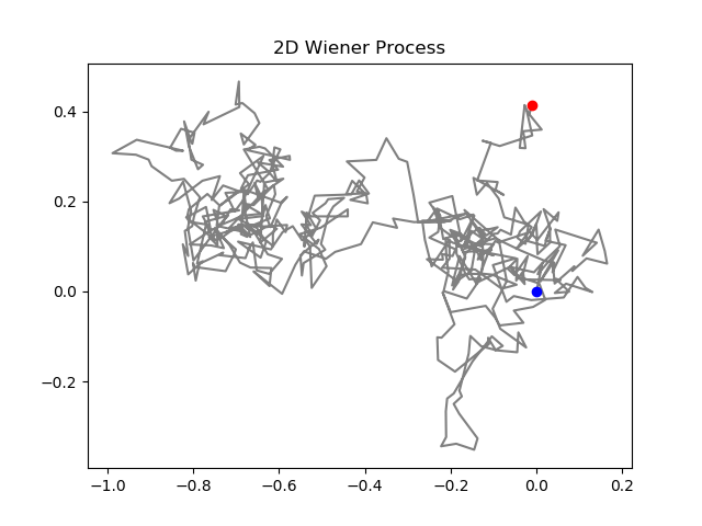
Throughout the rest of the diagrams, the blue point represents the start of a process while the red represents the end of the process.
| No Noise Random Walk | Random Walk |
|---|---|
 |  |
The left picture represent the left portion (after the equal sign) of equation 1, essentially what our “random” walk will look like if there was no noise or randomness. The right side is the exact opposite, it’s a random walk with no behavior toward a centralized point.
The OU process puts these two random walks together to produce stochastic random walk with a tendency toward a centralized point (in this case 0,0).

So what is the gaussian looking density that we’re seeing here? The cool thing about the OU process is that it has a tractable stationary distribution. In other words we can assign a probability density to any point on our space. Skipping the derivation, we can look at the probability density function. $$ p(x) = (2 \pi)^{-\frac{N}{2}}*det(\mathbf{A})^{-\frac{1}{2}}*exp(-\frac{1}{2} x^T \mathbf{A}^{-1} x)$$ where $$\mathbf{\beta A} + \mathbf{A \beta^T} = \mathbf{\Sigma\Sigma^T}$$
The probability density implies that OU path will tend to converge to the center. Interesting enough though, looking at the figure directly above, the random walk seems to orbit the center of the gaussian, which (if we assume SGD and OU are coupled) is what the authors of SWA noted. But why is this happening?
Well intuitively we have two vector forces acting on our point during a point in time. One being a force pulling toward our center and the second being a random Brownian motion. Let’s visualize the two vector forces to see what is happening near the orbit of our random walk.
So what’s happening here? As we got closer to the 0 point $-\beta \mathbf{x}_t dt$ tends to 0 leaving the major force behind the movement of our particle the Wiener process, which due to its property of independence, has the same expected magnitude of vector regardless of position on the field. In other words the magnitude of our noise vector stays the same while the informative vector disappears as it gets close to its centralized point.
So as we get closer the to the dense section of our p(x) the random noise kicks us out and then we tend to the center again and we repeat throughout the lifetime of the random walk.
This is very interesting behavior. You might be wondering why we’re spending time exploring this process so let’s connect SGD with the OU process before moving on with our analysis.
Representing SGD as an Ornstein-Uhlenbeck Process
The first paper (that I’m aware of) that represented SGD as an OU process was Stochastic Gradient Descent as Approximate Bayesian Inference by Mandt et al. We’ll follow the assumptions and derivations of the paper hopefully with more commentary. Let’s say we have a loss function that depends on the parameters of some function, over our complete training data. $$\mathbb{L}(\theta) = \frac{1}{M} \sum_{i=1}^{M} \mathbb{\ell}(\theta ; i), \ g(\theta) = \nabla_{\theta} \mathbb{L(\theta)} \ \ \ \ \bf{(3)}$$ We’re leaving out the actual function used because that’s not really of interest to us, but we can definitely rewrite the loss like so $\mathbb{\ell}(\theta ; i) = \mathbb{\ell}(f(x_i; \theta), y_i)$, it’s just more verbose plus we’ll be working with the loss landscape exclusively. Now generally we don’t take gradient steps utilizing a gradient over the whole training data. Instead we form a minibatch that’s uniformly sampled over our dataset. Let $\mathcal{S}$ be a set of random indices drawn uniformly from 1 to $M$, we can then get an unbiased estimate of our gradient via $$\hat{L_{\mathcal{S}}}(\theta) = \frac{1}{S} \sum_{i\in S} \mathbb{\ell}(\theta ; i), \ \hat{g_{\mathcal{S}}}(\theta) = \nabla_{\theta} \hat{\mathcal{L}_{\mathcal{S}}}(\theta) \ \ \ \ \bf{(4)}$$
Notice because $\hat{g_{ \mathcal{S}}}(\theta)$ is an unbiased estimator of $g$ we have in expectation $$g(\theta) = \mathbb{E}\left[ \hat{g_{ \mathcal{S}}}(\theta) \right] \ \ \ \ \bf{(5)}$$ We can then use this estimated gradient in our SGD update step. $$\theta(t+1) = \theta(t) - \epsilon \hat{g_{\mathcal{S}}}(\theta(t)) \ \ \ \ \bf{(6)} $$ Let's first try to figure out how we can derive the random noise portion of the OU process. Notice that increments of the Wiener process are Gaussian in nature. Furthermore the stochastic gradient is the sum of independent, uniformly sampled samples. We can therefore utilize central limit theorem to approximate the gradient noise with a Gaussian. $$g(\theta) =\hat{g_{\mathcal{S}}}(\theta) +\frac{1}{\sqrt{S}} \triangle g(\theta), ; \triangle g(\theta) \sim \mathcal{N}(0, C(\theta))\ \ \ \ \bf{(7)}$$ where $C(\theta)$ is a function that provides us with the covariance at $\theta$
Now lets make another assumption; the neighborhood we are considering is small enough so that we can approximate the covariance by a single positive definite matrix $C(\theta) \approx \mathbf{\Sigma} = \mathbf{\Sigma\Sigma^T}$.
Well if this is true our gradient approximation becomes the following equation. $$g(\theta)=\hat{g_{\mathcal{S}}}(\theta) +\frac{1}{\sqrt{S}} \triangle g(\theta), \ \triangle g(\theta) \sim \bf{\Sigma}\mathcal{N}(0,\mathbf{I})\ \ \ \ \bf{(8)}$$ And by rearranging equation 6 and plugging in equation 8 we get $$\theta(t+1)- \theta(t) = - \epsilon \left[g(\theta) - \frac{1}{\sqrt{S}}\bf{\Sigma}\mathcal{N}(0, \mathbf{I}) \right] \ \ \ $$ $$\triangle \theta(t) = - \epsilon g(\theta) + \frac{\epsilon}{\sqrt{S}}\bf{\Sigma}\mathcal{N}(0, \mathbf{I}) \ \ \ \ \bf{(9)}$$ Now if we can make the assumption that we can approximate our finite difference equation with a continuous stochastic DiffEq, we can rewrite our finite difference equation to $$d\theta_t = - \epsilon g(\theta) dt + \frac{\epsilon}{\sqrt{S}}\mathbf{\Sigma} dW(t)$$ Okay, we're almost there. The only thing left to do is to rewrite $g(\theta)$ via linear transformation of $\theta$. Without loss of generality let's say $\mathcal{L}(0) = 0$. Let's also assume that we can approximate the loss with a quadratic approximation. We then get $$\mathcal{L}(\theta) = \frac{1}{2}\theta \mathbf{H} \theta^T$$ where $\mathbf{H}$ is the Hessian at the optimum. Our final equation for SGD now is exactly the OU equation we described in the previous section. $$d\theta_t = - \epsilon \mathbf{H} \theta(t) dt + \frac{\epsilon}{\sqrt{S}}\mathbf{\Sigma} dW(t) \ \ \ \ \bf{(10)}$$
What can we say about SGD?
It's important that any intuitions we get by analysing the OU process be within our assumptions, the biggest being that we approximate the covariance and loss surface. Our approximations only make sense when we are within a small area of the loss surface. This tends to be the case only when we're toward the end of training.
The peculiarities we saw with the OU process, specifically the instability at the center of the OU process also apply to SGD. SGD seems to not be able to enter wide and flat minimas because the noise parameter that is derived from the stochasticity of the gradient, overpowers any information carried by the gradient. The balance is only restored around the boundary of the flat minima which is exactly what the SWA paper empirically showed.
So how does SWA solve this issue? Well by averaging points around the boundary of minima we'll end up in the center of the flat and wide minima (we denote this with a black point on the OU process figure above). The averaging of parameters is done when training is completed and no extra gradient updates are applied after the averaging. This makes perfect sense now since a gradient update might have enough noise to push the point out of the flat and wide minima.