Thu May 30, 2019 · 2830 words · 15 min

There was a interesting paper released some time in the past couple of weeks that showed it’s possible to do lossless compression via flow-based models. Historically flow based models didn’t get as much attention as VAE and definitely not as much as GAN’s so I paid very little mind to them. But flow based generative models exhibit very interesting properties and now the ability to do lossless compression warrants a deeper look into them. This post is rather large and therefore is split up into three sections. We’ll first introduce flow-based models, then we’ll discuss the various coupling layers we can define and lastly we’ll discuss how we can do lossless compression via neural networks.

The fundamental problem of generative modeling is learning a density $p(\mathbf{x})$ over some natural distribution. Furthermore a necessary condition for our generative model is that we have a efficient sampling strategy $x \sim p(\mathbf{x})$.

In order to be able to sample from $p(\mathbf{x})$ many generative models attempt to learn a function from a known prior distribution $p(\mathbf{z})$ to the natural distribution $p(\mathbf{x})$.

For example VAE's explicitly parameterize the output of the encoder to be standard normal via the reparameterization trick. GAN's on the other hand directly take a sample from a prior distribution (standard normal most of the time) as an input to the generator.

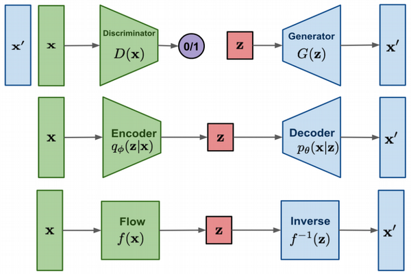
But what if we could devise a function $f(\mathbf{x})$ that maps from our natural distribution to our prior but also has the extra property that it is bijective (permits an inverse for every sample in it's range)?

Let's assume that we can find such a function what would could we do with it? Let's start off by formalizing some of the elements we've introduced so far.

Let $\mathbf{x},\mathbf{z} \in \mathbf{R}^n$, furthermore let's define the respective probability density functions: $\mathbf{x}\sim p(\mathbf{x}), \mathbf{z}\sim \pi(\mathbf{z})$. Lastly let's say that function: $$f: \mathbf{R}^n \rightarrow \mathbf{R}^n ; \ \ \mathbf{z} = f(\mathbf{x}) \ \ \ (1)$$

We can couple the two probability distributions with the continuous change of variable formula. $$p(\mathbf{x}) = \pi(\mathbf{z}) \left| \det \frac{\displaystyle d\mathbf{z}}{\displaystyle d\mathbf{x}}\right|, \text{for } \mathbf{z} = f(\mathbf{x}) \ \ \ (2)$$ And we can use the coupling $f$ to get $$p(\mathbf{x}) = \pi(f(\mathbf{x})) \left| \det \frac{\displaystyle df(\mathbf{x})}{\displaystyle d\mathbf{x}}\right|\ \ $$ or in log land $$\log{p(\mathbf{x})} = \log{\pi(f(\mathbf{x}))} + \log{\left| \det \frac{\displaystyle df(\mathbf{x})}{\displaystyle d\mathbf{x}}\right|}\ \ \ (3)$$

where $\frac{\displaystyle df(\mathbf{x})}{\displaystyle d\mathbf{x}}$ is the Jacobian of $f$ at $\mathbf{x}$. Recall that our Jacobian will be a real matrix of size $n \times n$

What we've done is made it possible to directly compute the log probability of our natural distribution through a differentiable bijective function. Therefore we can use standard negative log-likelihood to train our generative model. $$\mathcal{L}(\mathcal{X}) = \displaystyle - \frac{1}{|\mathcal{X}|} \sum_{\mathbf{x} \in \mathcal{X}} \log{p(\mathbf{x})}\ \ \ (4)$$ where $\displaystyle \mathcal{X}$ represents our training dataset. Furthermore sampling $x \sim p(x)$ is straightforward via $$ x = f^{-1}(z) \ \ \ (5)$$

Being able to directly optimize towards the log probability of our training set is an incredibly powerful tool. But the assumptions we made and the derived equations are rather intimidating. First, our coupling function needs to be bijective and easily invertible. Furthermore, equation 4 requires calculating an expensive determinant which has an asymptotic runtime of $\mathcal{O}(n^3)$.

The good news is, is that by carefully constructing our coupling function we can not only satisfy the necessary conditions but reduce the computational complexity of calculating the determinant. Let's enumerate the problems that we have to face.

Calculating the jacobian determinant $\displaystyle \det \frac{\displaystyle df(\mathbf{x})}{\displaystyle d\mathbf{x}}$ for a non-constrained function $f$ is non trivial.
Selecting a family of functions $f$ that is bijective.
Inverse of our functions $f^{-1}$ must be easily computable.

Bijective Transforms with Tractable Jacobian Determinants

The first paper I read that tackled this problem is Non-linear Independent Components Estimation by Dinh et al. So we'll follow along with their work as well as introduce some other forms of transforms that satisfy the conditions laid out at the end of the previous section.

The key fact that we'll use is that the determinant of a triangular matrix is equal to the product of diagonal elements.

Meaning that if we can construct our function in such a way that it's Jacobian $\frac{\displaystyle df(\mathbf{x})}{\displaystyle d\mathbf{x}}$ is a triangular (either upper or lower) matrix then the computationally expensive determinant becomes a fairly cheap operation.

$$\log{ \left| \det \frac{\displaystyle df(\mathbf{x})}{\displaystyle d\mathbf{x}}\right|} =$$

$$ \ \ \ \ \ \log{ \displaystyle \prod_{i=1}^{n} \left| \frac{\displaystyle df(\mathbf{x})}{\displaystyle d\mathbf{x}}\right|}_{i,i} = $$

$$ \ \ \ \ \ \ \ \ \ \ \ \ \displaystyle \sum_i^{n} \log{ \displaystyle \left| \frac{\displaystyle df(\mathbf{x})}{\displaystyle d\mathbf{x}}\right|}_{i,i}\ \ \ (6)$$

General Coupling Layer

Recall that $\mathbf{x} \in \mathbf{R}^n$. Let's also say that $d : d \le n$. Let's also say that $\displaystyle \mathbf{x_{1:d}}$ represents taking the first $d$ elements of $\mathbf{x}$ and $\displaystyle \mathbf{x}_{d:}$ represents taking all elements starting from element $d$.

using out new notation $$ \begin{equation} \begin{split} y_{1:d} &= x_{1:d},\ \ \ \ y_{d:} &= g(x_{d:}; m(y_{1:d}))\ \ \ (7) \end{split} \end{equation} $$ where $g: \mathbf{R}^{n-d} \times m(\mathbf{R}^d) \rightarrow \mathbf{R}^{n-d}$ The Jacobian and it's determinant will then be

$$\frac{\displaystyle d\mathbf{y}}{\displaystyle d\mathbf{x}} = \begin{bmatrix} I_d & 0 \\\frac{\displaystyle d\mathbf{y}_{d:} }{\displaystyle d\mathbf{x}_{1:d}} & \frac{\displaystyle d\mathbf{y}_{d:}}{\displaystyle d\mathbf{x}_{d:}} \end{bmatrix}, \ \det{\frac{\displaystyle d\mathbf{y}}{\displaystyle d\mathbf{x}}} = \det{\frac{\displaystyle d\mathbf{y}_{d:}}{\displaystyle d\mathbf{x}_{d:}}}\ \ \ (8)$$

where $I_d$ is the identity matrix of size $d$. The inverse of this function will then be \begin{align} y_{1:d} = x_{1:d}, \ \ \
y_{d:} = g^{-1}(x_{d:}; m(y_{1:d}))\ \ \ (9) \end{align}

What's cool is that we have no limitations on function $m$ and therefore we can parameterize it with a standard neural network with arbitrary complexity.

Additive Coupling Layer

$$g(a, b) = a + b$$

So our non-identity function will be:

$$\mathbf{y}_{d:} = \mathbf{x}_{d:} + m(\mathbf{y}_{1:d})\ \ \ (10)$$

even cooler is that our inverse function is as easy to compute as our forward function

$$\mathbf{x}_{d:} = \mathbf{y}_{d:} - m(\mathbf{y}_{1:d}) = \mathbf{y}_{d:} - m(\mathbf{x}_{1:d})$$

Furthermore our Jacobian will be lower triangular. This follows from

$$\displaystyle \frac{\displaystyle d\mathbf{y}_{d:}}{\displaystyle d\mathbf{x}_{d:}} = I_{n-d}$$

Therefore the determinant of this transform will always be 1, since our full jacobian is a lower triangular with only 1's on the diagonal.

Affine Coupling Layer

The additive coupling layer has a unit jacobian (i.e. volume preserving). This limits the level of expressiveness of this coupling layer, even if we stack multiple transforms on top of eachother. The original paper introducing additive coupling layers proposed a solution to this problem based on rescaling. But let's see if we can construct a transform that is more expressive.

$$\mathbf{y}_{1:d} = \mathbf{x}_{1:d}\ \ \ $$ $$\mathbf{y}_{d:} = \mathbf{x}_{d:} \circ \exp \left [ s(\mathbf{x}_{1:d})) \right ] + t(\mathbf{x}_{1:d}) \ \ \ (11)$$

Our Jacobian for this transform will be

$\frac{\displaystyle d\mathbf{y}}{\displaystyle d\mathbf{x}} = \begin{bmatrix} I_d & 0 \\\frac{\displaystyle d\mathbf{y}_{d:} }{\displaystyle d\mathbf{x}_{1:d}} & diag(\exp{s(\mathbf{x}_{1:d})}) \end{bmatrix} \ \ \ (12)$

As we can see from here the Jacobian is lower triangular, non volume preserving and we can use our shortcut to calculate the determinant inexpensively. This coupling layer was introduced by a follow up paper by Dinh et al titled [Density Estimation using Real NVP](https://arxiv.org/abs/1605.08803).

Combining Coupling Layers

Although a single coupling layer can be powerful, it makes sense that we might want to stack coupling layers to increase their expressiveness even more. Also note that the general coupling form keeps a portion of the input unchanged. But before going deeper on how to deal with this issue let's formalize exactly what it means to stack coupling layers.

We need to verify 3 things. Composition of function, determinant, inverse function.

$$ \text{Linearity of Differential Operator: } \frac{\displaystyle f_a \circ f_b}{ \displaystyle dx_a} (x_a) = \frac{\displaystyle df_a}{ \displaystyle dx_a} (x_a) * \frac{\displaystyle f_b}{ \displaystyle dx_b} (f_a(x_a)) \ \ \ $$ $$ \text{Determinant of Matrix Product: } \det{AB} = \det(A)\det(B) \ \ \ $$ $$ \text{Inverse of Composite Bijection: } (f_b \circ f_a)^{-1} = f_a^{-1} \circ f_b^{-1} \ \ \ $$

We'll leave the proof for these to Google, but these three rules provide us with a way to efficiently calculate Jacobian and inverse given a composition of our coupling layers. Now getting back to the problem at hand, which is that coupling layers in the general form provided do not augment a set of the original input. One trivial solution is to alternate across layers which portions of the input are passed through and which are changed. If we're working with images we can imagine more complicated masking schemes.

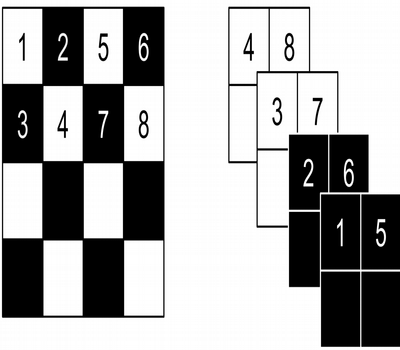
"Masking schemes for affine coupling layers. On the left, a spatial checkerboard pattern mask. On the right, a channel-wise masking." Source: Density Estimation using Real NVP ~ Figure 3.

Another layer introduced by the Real NVP paper was the Squeeze layer which reshapes the the image on the left into the image on the right. Directly from the paper: "The squeezing operation reduces the 4 × 4 × 1 tensor (on the left) into a 2 × 2 × 4 tensor (on the right). Before the squeezing operation, a checkerboard pattern is used for coupling layers while a channel-wise masking pattern is used afterward."

Lossless Compression

Hoogeboom et al released a paper recently titled Integer Discrete Flows and Lossless Compression. In this paper they introduce a new type of coupling that works directly off of discrete integers and because couplings are invertible it's possible to invert a discrete representation learned back into the original source. Now because we have theoretic guarantees on invertibility we can start to work toward learned lossless compression.

Figure 3 ~ Integer Discrete Flows and Lossless Compression.

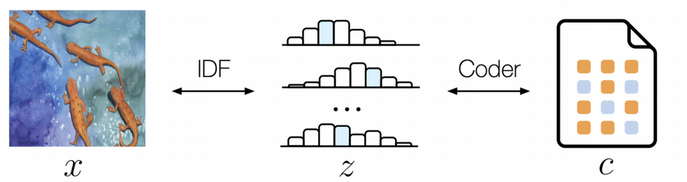
Recall that all types of flow-based generative models produce an output that has the same dimensions as the input, so naturally no trivial compression happens. But what Hoogeboom et al do is use a rANS entropy encoder to compress the discrete output given by the discrete flow model. Since both the discrete flow based model and rANS encoder are invertible we have an learnable end to end loss-less compression pipeline.

The papers contributions are that an easily invertible discrete coupling joined with a smart choice of prior can lead to a representation that can be effectively compressed using an entropy encoder. They showed serious compression gains over other lossless method.

Integer Discrete Coupling

The first step is understanding the design behind the discrete coupling. For this we'll have to update our definitions of variables.

Let $\mathbf{x} \in \mathbf{Z}^n$, the set of integers. Still using the general coupling formula we have:

$$ \mathbf{y}_{1:d} = \mathbf{x}_{1:d}$$ $$ \mathbf{y}_{d:} = \mathbf{x}_{d:} + \left\lfloor t(\mathbf{y}_{1:d})\right\rceil $$

where $\left\lfloor t(\mathbf{y}_{1:d})\right\rceil$ is rounding to the nearest integer the output from a neural network $t(\cdot)$. One problem that immediately jumps out is that the rounding operator is not differentiable. One way to get around this is to use the Straight-Through Estimator, which for the rounding operator will make us just skip the rounding operator in the backpropagation step:

$$ \nabla_{t(\mathbf{y}_{1:d})} \left\lfloor t(\mathbf{y}_{1:d})\right\rceil \triangleq\ \ \ \mathcal{I} $$

where $\mathcal{I}$ is the identity function.

Recall the additive coupling layer we introduced a couple sections back, integer discrete coupling is almost identical in the forward pass, and exactly identical in the backward pass. Interestingly enough Hoogeboom et al argue that even though the transform has a unit determinant (volume preserving) it's representative power when stacked is good enough. In general I haven't seen a consensus on what coupling layers work best in what scenario and I haven't read anything on theoretic guarantees of expressive power of coupling layers. This is a good future research direction.

Choice Of Prior

The authors choice for the prior distribution was a factored discretized logistic distribution.

$$ \pi(z | \mu, s) = \displaystyle \int_{z- \frac{1}{2}}^{z+\frac{1}{2}} \text{Logistic}(z' | \mu, s) \mathbf{d}z' = \sigma(\frac{\mathbf{z} + \frac{1}{2} - \mu}{s}) - \sigma(\frac{z - \frac{1}{2} - \mu}{s}) \ \ \ (13) $$

where $\sigma(\cdot)$ is the standard sigmoid function. Furthermore instead of having a static mean $(\mathbf{\mu})$ and scale $ (\mathbf{s})$ the authors parametrize them using a neural network.

Notice our choice of prior so far is unimodal. To fix this issue the authors use a mixture of discretized logistic distributions.

$\pi(\mathbf{z} | \mathbf{\mu}, \mathbf{s}) =\displaystyle \sum_{k=0}^{K} \alpha_k \pi(\mathbf{z} | \mathbf{\mu_k}, \mathbf{s_i}) \ \ \ $$

The authors note that a mixture of about 5 distributions was enough.

Architecture

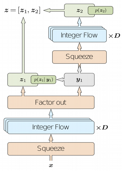
Figure 4 ~ Integer Discrete Flows and Lossless Compression. Example of a 2-level flow architecture. The squeeze layer reduces the spatial dimensions by two, and increases the number of channels by four. A single integer flow layer consists of a channel permutation and an integer discrete coupling layer. Each level consists of D flow layers.

"The IDF architecture is split up into one or more levels. Each level consists of a squeeze operation, D integer flow layers, and a factor-out layer. Hence, each level defines a mapping from $y_{l-1}$ to $\left[z_l, y_l\right]$, except for the final level L, which defines a mapping $y_{L-1} \rightarrow z_L$. Each of the D integer flow layers per level consist of a permutation layer followed by an integer discrete coupling layer. In the case of compression using an IDF, the mapping $f: \mathbf{x} \rightarrow \mathbf{z}$ is defined by the IDF. Subsequently, $\mathbf{z}$ is encoded under the distribution $p_Z(\mathbf{z})$ to a bitstream $c$ using an entropy encoder. Note that, when using factor-out layers, $p_Z(\mathbf{z})$ is also defined using the IDF. Finally, in order to decode a bitstream $c$, an entropy encoder uses $p_Z(\mathbf{z})$ to obtain $\mathbf{z}$. and the original image is obtained by using the map $f^{-1}: \mathbf{z} \rightarrow \mathbf{x}$, i.e., the inverse IDF."

The result for lossless compression are substantially better than our current methods and show the power of learned lossless compression.

igure 6 ~ Integer Discrete Flows and Lossless Compression.

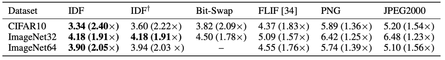
Results are in bits per dimension.

Conclusion

In conclusion we went in depth into flow-based generative models, various coupling layers that we can use and then lightly covered how we can learn to do lossless compression. The future of flow-based models is really interesting and the various benefits of flow-based models, specifically the tractable log probability, make it very attractive for a set of generative tasks.

If you're new to flow-based generative modeling I would highly recommend reading the papers in order as they are linked in this blog. But hopefully reading this provided you with the basic knowledge for understanding flow-based models!